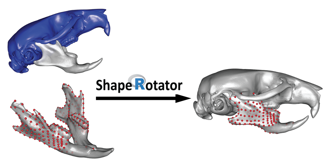
ShapeRotator - an R tool for standardised rotations of 3D structures
Welcome to the ShapeRotator Wiki!
In this Wiki I illustrate the functions available within the ShapeRotator R tool and the basic steps required in order to successfully implement the rotation on a dataset of 3D coordinates. ShapeRotator allows the rigid rotation of sets of both landmarks and semilandmarks used in geometric morphometric analyses, enabling morphometric analyses of complex objects, articulated structures, or multiple parts within an object or specimen.
You can now download the ShapeRotator R package from CRAN.
| shaperotator.pdf |
Citation:
Vidal-Garcia, M., Bandara, L. and Keogh, J.S. 2020. ShapeRotator: Standardised Rigid Rotations of Articulated Three-Dimensional Structures. R package version 0.1.0. https://CRAN.R-project.org/packages/ShapeRotator/
Vidal-García, M., Bandara, L. and Keogh, J.S. 2018. ShapeRotator: an R tool for standardised rigid rotations of articulated Three-Dimensional structures with application for geometric morphometrics. Ecology and Evolution. 8:4669–4675.
ShapeRotator R code:
ShapeRotator R code:
You can download an example file for simple.rotation() and double.rotation()
| example_simple_rotation.r |
| example_double_rotation.r |
You can now download the ShapeRotator R package from CRAN:
install.packages("ShapeRotator")
library(ShapeRotator)
Importing a dataset:
We first import the two datasets to joing using the R package geomorph:
library(geomorph)
For example, if we wanted to import a tps file we would do the following:
data_1 <- readland.tps(“data_1.tps”, specID = “ID”, readcurves = F)
data_2 <- readland.tps(“data_2.tps”, specID = “ID”, readcurves = F)
For more help on importing the GM datasets, please see Adams et al. (2017) and the associated help files in geomorph. Please note that this method also works for semilandmarks.
Selecting landmarks and rotation axes:
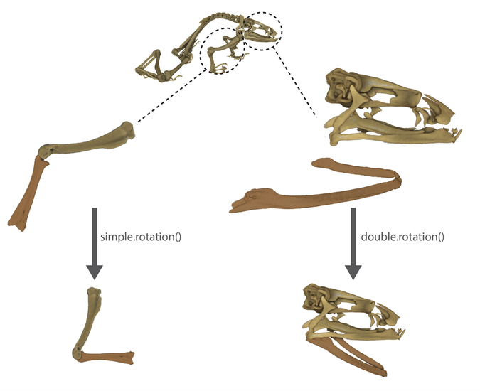
You will need to select different number of landmarks and the associated rotation axes depending on whether you would like to perform a simple.rotation() OR a double.rotation()
install.packages("ShapeRotator")
library(ShapeRotator)
Importing a dataset:
We first import the two datasets to joing using the R package geomorph:
library(geomorph)
For example, if we wanted to import a tps file we would do the following:
data_1 <- readland.tps(“data_1.tps”, specID = “ID”, readcurves = F)
data_2 <- readland.tps(“data_2.tps”, specID = “ID”, readcurves = F)
For more help on importing the GM datasets, please see Adams et al. (2017) and the associated help files in geomorph. Please note that this method also works for semilandmarks.
Selecting landmarks and rotation axes:
You will need to select different number of landmarks and the associated rotation axes depending on whether you would like to perform a simple.rotation() OR a double.rotation()
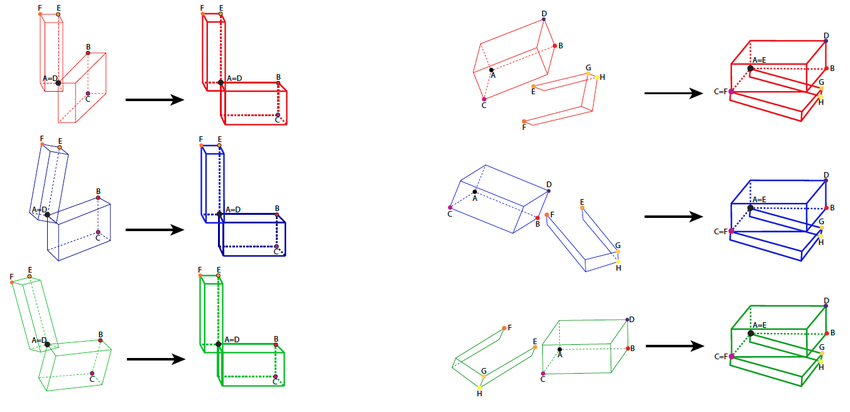
For simple.rotation() each structure needs to have three selected landmarks: landmarks A, B, C for data_1 and landmarks D, E, F for data_2. For double.rotation() we will need an extra landmark (landmarks A, B, C, D for data_1 and landmarks E, F, G, H for data_2).
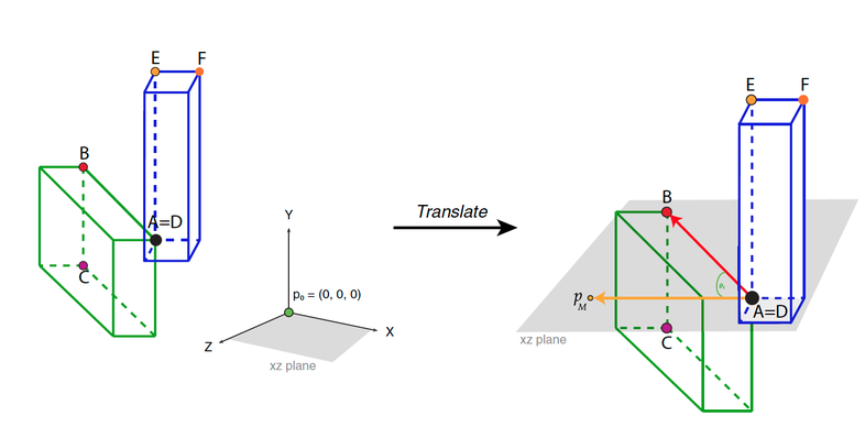
Translating:
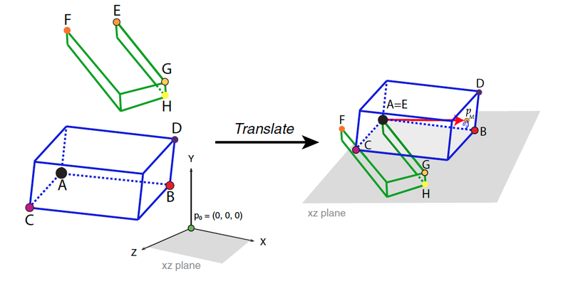
During this step, each structure will be translated to the point of origin so that ̃p0 =(0,0,0).We will be translating landmark A from structure 1 and landmark D from structure 2 for a single-point articulated rotation, and landmark A from structure 1 and landmark E from structure 2 for a double rotation (double-point articulated rotation). Thus, the distance from the coordinates of landmark A (Ax, Ay, Az) is substracted from all the landmarks in all specimens, for example (Nx − Ax, Ny – Ay, Nz – Az) for landmark N, for structure 1. For structure 2, the distance from the coordinates of landmark D or E depending on the type of rotation. For example, in a double rotation, (Ex, Ey, Ez) is substracted from all the landmarks in all specimens: (Nx − Ex, Ny – Ey, Nz – Ez). Landmarks A and E will equal (0,0,0), so that Ax=Ay=Az=Ex=Ey=Ez=0. This translation is made with the function translate().
Translation for a single-point articulated structure:
For the first dataset: data1_t <- translate (T = data_1, landmark = landmark_A)
For the second dataset: data2_t <- translate (T = data_2, landmark = landmark_D) for the simple.rotation()
Translation for a double-point articulated structure:
For the first dataset: data1_t <- translate (T = data_1, landmark = landmark_A)
For the second dataset: data2_t <- translate (T=data_2, landmark = landmark_E) for the double.rotation()
Please note that the default is to set the origin point to, but this can be changed to another origin point. For example, to the point c(1, 3, 5):
data1_t <- translate (T=data_1, landmark=landmarkA, origin = c(1,3,5))
data2_t <- translate (T=data_2, landmark=landmarkD, origin = c(1,3,5))
Rotating the translated datasets
Simple rotation
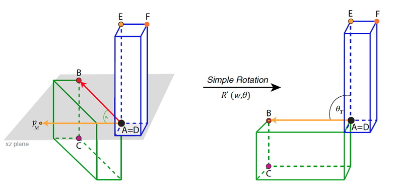
Rotation method exemplified for simple.rotation() by depicting the plane spanned by the already translated point p0 and A. Please note that p0 depicts the origin point (0, 0, 0). The rotated resulting point pM, landmarks B, C, D, E, and F, and angle θT (desired angle between the two structures) are also depicted:
In the rotation step, we will use the function simple.rotation() in order to rigidly rotate the two structures of example A to the desired angle (in degrees), as it follows:
rotated_dataset <- simple.rotation(data.1 = data1_t, data.2 = data2_t, land.a = 10, land.b=1, land.c=17, land.d=52, land.e=19, land.f=107, angle = 90)
The input datasets data.1 and data.2 correspond to the two translated datasets. We then use the selected landmarks as explained in the previous section. Finally, we include the angle (in degrees) that we would like to use to position the two structures to one another.
This file (rotated_dataset) has two parts (rotated_dataset$rotated1 and rotated_dataset$rotated2) which correspond to the rotated data_1 and data_2. In order to obtain the final rotated dataset, we need to join them:
joined_rotated_dataset <- join.arrays(rotated_dataset$rotated1, rotated_dataset$rotated2)
Then we can plot in a 3D scatterplot the joined dataset with the rotated two structures:
plot.rotation.3D(joined_rotated_dataset, data1, data2, specimen.num = 1)
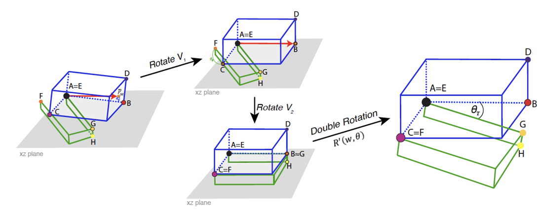
Double rotation
Similarly to simple.rotation(), the double.rotation()will be as follows:
double_rotated_dataset_45 = double.rotation(data.1= data1_t, data.2= data2_t, land.a=1, land.b=2, land.c=3, land.d=4, land.e=1, land.f=2, land.g=3, land.h=4, angle=45)
Even though each of these rotations are calculated internally (only the four landmarks per structure and the desired angle between them need to be provided), it will be beneficial to choose landmarks that are spatially arranged in a way that facilitates the rotation process, and results in the rotating multi-structure being placed in a biologically-relevant angle between each sub-structure. ShapeRotator will give a warning message if the landmarks chosen are not optimal.
The function double.rotation() will return a list of two elements (double_rotated_dataset_45$rotated1, double_rotated_dataset_45$rotated2) that will need to be joined as it follows:
joined_double_rotated_dataset_45 = join.arrays (double_rotated_dataset_45$rotated1, double_rotated_dataset_45$rotated2)
Double.rotation() allows the user to translate one of the objects after the rotation, in the case of not wanting them in contact to one another. For example, if it would me anatomically more correct to have the second structure translated to point c(1.7, 0.1, 0): skull_translate = c(1.7,0.1, 0)
joined_double_rotated_dataset_45_t = join.arrays (double_rotated_dataset_45$rotated1, translate(double_rotated_dataset_45$rotated2,land.e, skull_translate))
Finally, after the rotation process we can visualize a 3D plot for each specimen with the two rotated structures for both a single-point and a double point articulations using the function plot.rotation.3D():
plot.rotation.3D(joined.data=joined_double_rotated_dataset_45_t, data.1=data_1, data.2=data_2, specimen.num =1)
The default plotting colours for the landmarks of the joined rotated structure (joined.data) is black and red for each original structure (data.1 and data.2).
Exporting the rotated (and joined) datasets
After the rotation process we could either use the joined GM array in further analyses, visualise the resulting joined structure through geomorph (Adams & Otárola-Castillo 2013), or we could also export it and save it in order to use it in another software, such as MorphoJ (Klingenberg 2011). In this step we will be using the function writeland.tps() in the R package geomorph (Adams & Otárola-Castillo 2013) in order to save a tps file from the joined GM array:
writeland.tps(A="joined_arm", file = " joined_arm.tps", ...)
